Inspired by a fellow YMH podcast (warning NSFW) fan/mommy, Eric, I am trying my hand at analyzing YMH podcast transcripts. I plan on following along with Eric’s work flow below and diverting once I find an opportunity to personalize the analysis - aka keeping it high and tight and following proto.
Based on the structure of Eric’s blog post, this analysis will proceed as follows:
Load R libraries
Test API call
Generate YMH URL list
Data cleaning
List API call
Finalize API call output
I don’t have any experience in pulling transcripts from YouTube or any serious text analysis so I’m excited to try it out. Thanks for not being stingy, Mark… I mean Eric!
Libraries
library(tidyverse)
library(youtubecaption)
library(janitor)
library(lubridate)
library(reshape2)
Aside from {tidyverse}, {reshape2}, and {lubridate}, Eric uses {youtubecaption} for calling YouTube’s API to get the caption transcripts and {janitor} for some of the text analysis, namely the clean_names() function. These two packages are brand new to me so I’m excited to work with them.
Note: I learned further into this analysis that {youtubecaption} relies on Anaconda, a comprehensive Python environment, to pull from YouTube’s API. The author of youtubecaption states the reason for this is due to the difficulty of calling YouTube’s API for the captain data in a user friendly format. Thus, this library acts as a handy and clean way of accessing YouTube’s API in Python (Anaconda) without needing to write a custom API call in another language. I didn’t have Anaconda on this machine so I had to take a break from the analysis to install Anaconda before running functions from that library. Save yourself some time and download it before getting started!
Test YouTube API call, episode 571
ymh_e571 <- get_caption("https://www.youtube.com/watch?v=dY818rfsJkk")
And there we go, a really straight forward way to download a transcript from a specific YouTube video. I can see why Eric used this package and that’s the easiest API call I’ve ever used. Let’s take a look at what we are working with:
head(ymh_e571)
A tibble: 6 x 5 segment_id text start duration vid
<int> <chr> <dbl> <dbl> <chr>
1 1 oh snap there’s hot gear 0.64 5.12 dY818rfsJkk
2 2 merch method dot com slash tom sagura 3.04 5.84 dY818rfsJkk
3 3 check out all our new stuff 5.76 3.12 dY818rfsJkk
4 4 these club owners will take advantage as 9.92 3.04 dY818rfsJkk
5 5 you know 12.2 2.40 dY818rfsJkk
6 6 if you don’t stand your ground i don’t 13.0 2.88 dY818rfsJkk
Upon inspection, the YouTube API call gives us 5 columns and just over 4500 rows or data. ‘Segment_id’ would be our unique identifier for each segment, ‘text’ is obviously the speech-to-text captions we are after, ‘start’ appears to be the time stamp when the text is recorded, the value of ‘duration’ is a mystery at the moment but we’ll look into that later, and ‘vid’ is simply the YouTube HTML video id (the characters after “watch?v=” in every YouTube video address).
The next step would be to download the transcripts for a number of episodes, but so far we’ve only made an API call to YouTube using the exact URL for a specific video. How are we going to call a list of videos outside of manually looking up all 571 YMH videos one at a time? Eric figured out a nice solution on his blog and we’ll explore it next.
Generate YMH URL list
What we can do to script out a large API call is take a YMH YouTube playlist and export that to a text file. From there, we have a full list of YMH videos, their names, and, most importantly, the URLs. There are plenty of web tools and extensions to export a YouTUbe data to a .csv and only require a quick Google search to find one. Eric used this tool which looks straight forward and conveinent. Once you have the list, we’ll need to clean and arrange the file to use when calling from the YouTube API.
Houston, we have a problem:

Turns out the web app Eric used to gather the YouTube playlist and episode information is no longer working. We will have to find other means of generating this list to make the API call. After a painstaking Sunday searching for alternative web apps and testing them, I was not able to find anything that fit the needs for this project. That is until I stumbled upon YouTube-dl, a command-line program created to download YouTube videos and/or audio tracks from YouTube and a host of other sites. Turns out this program can also be used to scrape the YouTube metadata of videos. It took some time (and reddit/r/youtube-dl threads) to figure out how to use the tool to generate a list of video titles and URLs from a playlist, but I come to you with the knowledge! So lets do this, shall we?
First thing you’ll want to do is download the youtube-dl .exe windows application from their site and place it into a folder. Open a cmd window and set that folder as your directory directory. Lucky for you, I’ve done all the troubleshooting and testing of this tool. These are the commands I decided to use, mainly due to my limited knowledge of the windows command line.
This command will result in a long csv file, with the episode title and url id all in one column:
youtube-dl.exe –flat-playlist –get-title –ignore-config –get-id -o
[“https://www.youtube.com/watch?v=%(id)s” “https://www.youtube.com/playlist?list=PL-i3EV1v5hLd9H1p2wT5ZD8alEY0EmxYD”,](“https://www.youtube.com/watch?v=%(id)s” “https://www.youtube.com/playlist?list=PL-i3EV1v5hLd9H1p2wT5ZD8alEY0EmxYD”,)>ymh_playlist.csv
Instead of dealing with the above output, I decided to just export two files, one with the playlist video titles and another with the playlist video url id’s and simply join them in R:
youtube-dl.exe –flat-playlist –get-title –ignore-config -o
[“https://www.youtube.com/watch?v=%(id)s” “https://www.youtube.com/playlist?list=PL-i3EV1v5hLd9H1p2wT5ZD8alEY0EmxYD”,](“https://www.youtube.com/watch?v=%(id)s” “https://www.youtube.com/playlist?list=PL-i3EV1v5hLd9H1p2wT5ZD8alEY0EmxYD”,)>ymh_title.csv
youtube-dl.exe –flat-playlist –get-id –ignore-config -o
[“https://www.youtube.com/watch?v=%(id)s” “https://www.youtube.com/playlist?list=PL-i3EV1v5hLd9H1p2wT5ZD8alEY0EmxYD”,](“https://www.youtube.com/watch?v=%(id)s” “https://www.youtube.com/playlist?list=PL-i3EV1v5hLd9H1p2wT5ZD8alEY0EmxYD”,)>ymh_id.csv
You should end up with either one or two .csv’s with a single column of data, depending on your preferred method. Let’s take a look at them:
playlist_title <- read.csv(“~/GitHub/blog_website_2.0/blog_data/ymh_title.csv”,
header=FALSE)
playlist_url <- read.csv(“~/GitHub/blog_website_2.0/blog_data/ymh_id.csv”,
header=FALSE)
head(playlist_title)
V1
1 Your Mom’s House Podcast - Ep. 572 w/ Chris Distefano
2 Your Mom’s House Podcast - Ep. 571 w/ Marcus King
3 Your Mom’s House Podcast - Ep. 570 w/ Ian Bagg
4 Your Mom’s House Podcast - Ep. 569 w/ Duncan Trussell
5 Your Mom’s House Podcast - Ep. 568 w/ Kevin Nealon
6 Your Mom’s House Podcast - Ep. 567 w/ Fortune Feimster
head(playlist_url)
V1
1 wTvMDkAZZnM
2 dY818rfsJkk
3 _VCG6PzLnRA
4 J4hQnfu9nkY
5 bGklkg3m-6U
6 zSRBGlyisno
Data Cleaning
We’ll do some reshaping and data cleaning next. Now I’m not the best person to explain data cleaning steps and I know there are probably simpler, faster, and more efficient ways of doing it but these worked for me. I’d suggest searching for some of the experts on {tidyverse} and {reshape2} to learn about it!
append_rows <- which(!(grepl(“Your”, playlist_title$V1)))
title_rows <- c(20, 20, 86, 98, 250, 251)
playlist_title[paste(title_rows, sep = “,”),] <- paste(playlist_title[paste(
title_rows, sep = “,”),], “,”,playlist_title[paste(
append_rows, sep = ","),])
playlist_title <- playlist_title %>% filter((grepl(“Your”, V1))) %>%
rename(“title” = V1)
playlist_url <- playlist_url %>% slice(1:245) %>% transmute(
[ url = paste(“https://www.youtube.com/watch?v=”, V1, sep = “”))]( url = paste(“https://www.youtube.com/watch?v=”, V1, sep = “”)))playlist_clean <- cbind(playlist_title, playlist_url)
playlist_clean <- playlist_clean %>%
clean_names() %>%
## systematically cleans any text or symbols up
separate(title, c(“title”, “episode”), “-“) %>%
## separate episode title by ‘-‘
mutate(vid = str_replace_all(url, “.=(.)$”, “\1”))
## creates a vid column of just the youtube short link, this column matches
## the “vid” output from get_caption() and will be used to join the two tables
glimpse(playlist_clean)
Rows: 245
Columns: 4
$ title
$ episode
[$ url
Success! We have 245 rows of observations of YMH episodes, #330 to #572, plus some extra/live episodes with titles and URLs. You’ll notice I tweaked some rows and cut off some rows in the cleaning steps. If you interrogate the data more, you’ll find that either the youtube-dl tool or the command line does not export data into a .csv. cleanly. I found some of the long YouTube titles ended up having part of the title placed on a second row. Also, the last 2 videos in the playlist are marked as deleted and/or private so I removed those as well.
Now we can start working on pulling the transcripts for the 245 episodes we’ve generated.
List API call
The next steps is to again use the get_caption() function again but this time we need the function to pull all the captions from the list of URLs. We also want to make sure the get_caption() function successfully runs through the list and alerts us to any video it cannot successfully call. The way Eric did this was to wrap the get_caption() function inside the safely() function from {purrr}.
?safely to read up safe_cap <- safely(get_caption)
Based on the help documents, safely() provides an enhanced output of errors, messages, and warnings outside of the base r reporting. This function should help determine if our large API call has an errors while running.
Within the same {purrr} library, the map() function applies a function to each element of a list. Therefore, in out case, map() will apply the get_caption() function to each URL in the playlist and, by wrapping safely() around get_caption(), will provide enhanced outputs and errors.
playlist_call <- map(playlist_clean$url,
safe_cap)
warning - large print out:## glimpse(playlist_call)
Finalizing the API call output
With the list API call finished, the return of the map() function resulted in a vector of the 245 captions. But instead of a single output, we have a result output and an error output from the safely() function and we want to get the ‘result’ outputs from each vector. (By the way, feel free to check those safely() error messages before continuing to see if you need to traceback anything).
To do this, we will again call the map() function as well as the pluck() function from {purrr} (you got to love these function names from a library called {purrr} :D). Pluck() essentially indexes a data structure and returns the desired object, in our case the resulting caption text from each URL.
playlist_data <- map(1:length(playlist_call),
                 ~pluck(playlist_call, ., "result")) %>%

                   compact() %>%

                   bind_rows() %>%

                   inner_join(x = playlist_clean,

                              y = .,

                              by = "vid")
glimpse(playlist_data)
Rows: 527,189
Columns: 8
$ title
$ episode
[$ url
$ segment_id
$ text
$ start
$ duration
Success! We’ve ended up with a table of 8 variables and over 500,000 segments of caption text. This is a good place to stop for now and we’ll pick back up on part 2 with the text analysis.
Thanks again to Eric Ekholm, blog post, who laid the foundation for me to learn this youtube api call process!
Part 2: the text analysis
Originally posted October 16, 2020.
I’m back, Jeans! For those who missed Part I of this two-part YMH analysis, I followed along with Eric Ekholm’s blog post to pull YouTube speech-to-text captions for a playlist of YMH videos. If you missed the warning, this is NSFW content so tread lightly all you cool cats and kittens.
Now that we have the YouTube text data, it’s time to dive in and see what we can learn about our pals Tom and Christine. Similar to Part 1’s blog post, I am going to follow along with Eric’s second YMH blog post where he analyzed this data and find opportunities to learn from him as well as unpack the data in other ways.
Before we get off on this analysis, there are a few important observations of the text data I should mention:
The episode transcripts are automatically created by Youtube’s speech-to-text model. It usually performs very well, but it does make some mistakes & obviously has trouble with proper nouns (e.g. TikTok).
The speakers of each phrase are not tagged or timestamped. That is, there are no indications whether Tom, Christina, or someone else are speaking any given line.
This should be fairly obvious at this point but I’m only looking at the episodes available on Youtube. The most recent episode included is episode 572 with Chris Distefano, aka Chrissy Drip Drop, aka Chrissy one-and-done, aka Chrissy vodka soda.
Alright we’ve feathered it enough, let’s get started with some data cleaning and manipulation.
Setup and data work
library(tidyverse)
library(lubridate)
library(tm) ## text mining
library(tidytext) ## text mining
library(tidylo) ## improved weights to lists, like top_n
library(igraph) ## edge sequencing
library(ggraph) ## ggplot2
library(vroom) ## improved csv reading & in line piping
library(reactable) ## interactive tables
library(plotly) ## interactive plots!!
library(wordcloud)
ymh <- vroom(“~/GitHub/blog_website_2.0/blog_data/ymh_data.csv”)
ymh_single_row <- ymh %>%
group_by(title, ep_no) %>%
summarise(text = str_c(text, collapse = “ “) %>%
str_to_lower()) %>%
ungroup()
Descriptives
Episode length
We have a total of 175 observations, or episodes, worth of data to investigate, ranging from episode 345 to 572. Let’s take a look at some descriptives about YMH episodes.
ep_length <- ymh %>%
group_by(ep_no) %>%
summarise(minutes = (max(start) + max(duration))/60) %>%
ungroup()
ggplotly(ep_length %>%
ggplot(aes(x = ep_no, y = minutes)) +
geom_point(color = “black”) +
geom_line(color = “black”) +
labs(
title = "YMH Episode Length",

x = "Episode Number",

y = "Length (mins)"
)
)
It looks like we have an outlier episode. If you hover over that point on the plot with your mouse/cursor (yes, these plots are interactive!), you will see there is a break between in subtitles generated by YouTube between approx. episode 330 and 394. Let’s go ahead and remove all episodes below 394 moving forward and try this again
ymh <- ymh %>% filter(ep_no > 393)
ep_length <- ymh %>%
group_by(ep_no) %>%
summarise(minutes = (max(start) + max(duration))/60) %>%
ungroup()
ggplotly(
ep_length %>%
ggplot(aes(x = ep_no, y = minutes)) +
geom_point(color = “black”) +
geom_line(color = “black”) +
labs(
title = "YMH Episode Length",

x = "Episode Number",

y = "Length (mins)"
)
)
That’s much better!
Looking at the second plot, it’s clear that around episode 450, the length of episodes began to increase to upwards of 250 minutes long (4 hours!) before plateauing at around 150 minutes. It’s interesting to see such wide variability in episode length, instead of more stepped/staggered changes. There are a lot of lows and highs among episode lengths, symptomatic of a person on Meth as Dr Drew would point out. With this much variability, let’s fit a smooth line to the plot to help identify more trends.
ggplotly(
ep_length %>%
ggplot(aes(x = ep_no, y = minutes)) +
geom_point(color = “black”) +
geom_line(color = “black”) +
geom_smooth(method = “loess”, formula = “y ~ x”, color = “blue”) +
labs(
title = "YMH Episode Length, Second Attempt",

x = "Episode Number",

y = "Length (mins)"
)
)
Ah, that looks better. So it looks like episode length hit it’s peak around episode 480 and smooths out at approximately ~150 minutes.
Guests
Guests, usually fellow comedians, are a huge part of the show. Let’s look into the official guests on the show. I say official because I am reliant upon the title to inform me who was a guest on the show. Regular characters like Tom’s parents, Dr Drew, and Josh Potter won’t show up in this figure.
ymh %>%
distinct(ep_no, .keep_all = TRUE) %>%
mutate(guests = str_replace_all(guests, “\&”, “,”)) %>%
separate_rows(guests, sep = “,”) %>%
mutate(guests, str_trim(guests)) %>%
filter(!is.na(guests)) %>%
count(guests, name = “num_appearances”, sort = TRUE) %>%
filter(num_appearances > 1) %>%
reactable()
Alright so not a big surprise to anyone that Tom’s best friend, Bert Kreischer, was the top guest here. I’m glad to see Nikki Glaser as number 3 on the list, for one reason because she is the only repeat female guest but she is also savagely hilarious. Overall, it’s pretty clear YMH does not have a lot of repeat guests (at least in in the most recent ~200 shows). You’ll notice I removed any guest who did not have more than 1 appearance to make the list more manageable.
Text Analysis
Word Usage
Moving past some of the descriptive data, lets get into the text analysis portion of this project - the result of all that YouTube API calling in Part I. I’ll be taking a lot cues from Eric’s blog post for this part since this will be my first time doing any serious textual analysis in R.
Just like in the limitations of guest count based on title, if you look at the YouTube text-to-speech data, it is not structured to show who is speaking when it records text. No matter, as you’ll see there is a lot of rich text and data in here to dig through.
The first step is to remove many of the common words in the English language like “the”, “at”, “I’m”, etc.
ymh_words <- ymh_single_row %>%
filter(ep_no > 393)%>%
unnest_tokens(word, text)
creates a token for each word in the single row text ## column we collapsed in the beginning of the post.
ymh_words <- ymh_words %>%
anti_join(stop_words) %>%
## anti_join = ! in that it returns the opposite of what we want.
## In this case, it returns all words that do not match with the stop_words
## function containing the entire lexicon of English common words like “the”
filter(!(word %in% c(“yeah”, “gonna”, “uh”, “hey”, “cuz”, “um”, “lot”))) %>%
## filtering out additional common YMH specific words
filter(!(is.na(word)))
ggplotly(
ymh_words %>%
count(word) %>%
slice_max(order_by = n, n = 20) %>%
## select the top 20 rows and order them
ggplot(aes(x = n, y = fct_reorder(word, n))) +
geom_col(fill = “red”) +
labs(
title = "Most Used YMH Words",

y = NULL,

x = "Count"
)
)
You have got to be ‘ing kidding me. Turns out that somehow Eric was able to download the raw/uncensored YouTube captions back in May and I’m stuck here with this . When I noticed I wasn’t finding any curse words, I went back and watched a few YMH clips and noticed that every time they cursed, the YouTube captions transcribed on the video closed captions. And, as you can see from the chart, they’ve essentially aggregated all curse words into one huge cluster- . Let’s see if we can still work around this and even use it to our advantage.
Aside from YouTube censoring of our analysis, we have a few other notable mentions in the top 20 words used. “People” is clearing the most used word, but we also see “guy”, “cool”, “crazy”, and “music”. YMH does have some incredibly talented fans with their music submissions to close out the episode, Hendawg for example, so “music” makes a lot of sense.
Wordcloud
The bar chart was a little boring and is limited to the top 20 words. Let’s look at a more nuanced text analysis visualization: Wordclouds. Turns out the {wordcloud} package makes these things trivial to recreate with a bit of formatting.
ymh_wc <- ymh_words %>%
count(word) %>% filter(!grepl(“[[a-z]]+”, word))
ymh_wc$word <- removePunctuation(ymh_wc$word)
Our curse word symbol “” won’t look right in the wordcloud so I opted to remove it
ymh_wc_p <- wordcloud(words = ymh_wc$word, freq = ymh_wc$n, min.freq = 1,
        max.words = 300, random.order = FALSE,

        colors = brewer.pal(8, "Set1"))
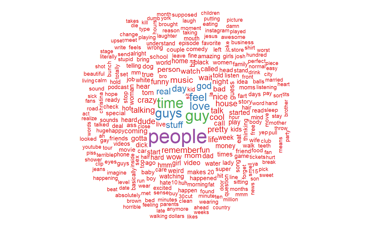
Even though we had to remove from the wordcloud (I could have replaced it with “curses” but we would just have a huge “curses” in the middle which isn’t very insightful), there are still some interesting words in here. One thing is for sure, I could increase the max.words() even higher than 300 and the takeaway here woudls till be that YMH has a wide vocabulary - not surprising for a podcast with almost 600 episodes.
Potty Mouths
Given that YouTube seems to have provided us with a curse word catch-all token, let’s see if we can use this to our advantage. In Eric’s blog post, he looked into number of “fuckings” per minute by episode. We can do the same thing here for .
quick note here: while writing this plot I kept getting “Error in annotate: unused arguments”## because both the {tlm} and {ggplot2} packages have annotate functions. To resolve that, I simply## force-called the ggplot2 function and it worked fine!
ggplotly(
ymh_words %>%
filter(word == “”) %>%
count(ep_no, word) %>%
left_join(ep_length, by = “ep_no”) %>%
mutate(cpm = n/minutes) %>%
ggplot(aes(x = ep_no, y = cpm)) +
geom_text(aes(size = cpm), label = “curses”,
        show.legend = FALSE, color = "black") +

ggplot2::annotate("text", x = 535, y = 3.39,

                  label = "- Ep. 494 w/ Joey 'Coco' Diaz",

                  hjust = 0, size = 3.5) +

ggplot2::annotate("curve", x = 494, xend = 500, y = 3.2,

                  yend = 3, curvature = .4) +
labs(
title = "'s per minute per YMH episode",

x = "Episode number",

y = "'s per minute"
)
)
Woah so here’s a shocker! Episode 494 with Joey Diaz blows away the other episodes! Episode 494 had nearly 3.5 curse words per minute, 50% more than the next closest episode (ep. 451 w/ Chris D’Elia) for a total of 460 curse words in just 2 hours. Funny enough, episode 516 with Donnell Rawlings and Grant Cardone had the last number of curses, just 26 (looks like a little spec just after 500 on the x-axis).
Catch Phrase Traceback
YMH is known for their catch phrases. Whether its “try it out”, “feathering in”, or “water champ”, the true mommies have a lot of inside jokes. Let’s see if we can traceback these jokes to when they first made appearances on the show. (Note: since we do not have a full collection of YMH episodes and the earlier episodes were audio only, we’ll only be able to traceback more recent phrases. I doubt we’ll be able to find the origin of “Jeans” or “Mommies” in here).
ggplotly(
ymh_words %>%
filter(word == “julia”) %>%
count(ep_no, word) %>%
left_join(x = tibble(ep_no = unique(ep_length$ep_no), word = “julia”),
y = ., by = c("ep_no", "word")) %>%
mutate(n = replace_na(n, 0)) %>%
ggplot(aes(x = ep_no, y = n)) +
geom_line(color = “black”, size = 1.25) +
labs(

title = "Good Morning, Julia!",

subtitle = "Counts of the word Julia per episode",

x = "Episode Number",

y = "Count")
) %>%
layout(title = list(text = paste0(“Good Morning, Julia!”,
                                "<br>",

                                "<sup>",

                                "Counts of the word Julia per episode",

                                "</sup>")))
The word Julia clearly saw a limited run on YMH. It peaked, dramatically, on episode 478 and was first mentioned on episode 432. Julia was last used during episode 556 so it hasn’t seen any action, so to speak, for about 20 episodes. That spike in episode 478 is interesting, though! Checking Eric’s blog post, it looks like that episode had Tom and Christina actually interview Julia. That makes a lot of sense in how the show runs, they probably locked down the interview a few episodes prior and hyped it up by playing the video a lot, which would explain the increase on episode 468. Afterwards, the word essentially lost popularity after the hype died out in the following episodes.
We aren’t stop here. There are a plenty of other words or phrases to try to traceback with this data. Eric, in his blog post, wrote a neat little function to extract a bunch of words/phrases and create a faceted graph. Let’s try that out. (As a personal note, I did not write this function, Eric did. I put in some time and effort to understand and explain it in the code chunk+ below but all credit for this function belongs to Eric.)
create the function phrase## for vector “nwords”, if the string count is 1 = word, else if it is not = 1 then = “nram”## (essentially a sequence of words, later identified as a phrase)## for “ngrams” split the ymh_single_row table into tokens, “n = nwords” for the phrases, else for the “words”## subset data in tpm which does not equal phrase function (i.e. does not equal the ‘phrases’ ‘vector)## create the phrase_list using the map() function and the i_phrase function based on the phrases vector
i_phrase <- function(phrase) {
nwords <- str_count(phrase, “ “) + 1
token <- if (nwords == 1) {
"words"
} else {
"ngrams"
}
tmp <- if (token == “ngrams”) {
ymh_single_row %>%

  unnest_tokens(output = words, input = text, token = token, n = nwords)
} else {
ymh_single_row %>%

  unnest_tokens(output = words, input = text, token = token)
}
tmp %>%
filter(words == phrase)
}
phrases <- c(“julia”, “feathering it”, “tick tock”, “let me eat”, “hitler”,
         "ride or die", "sleep for three days", "face fart",

         "new relationship energy", "cool guy", "milligram tom", "badly")
ymh_phrase_list <- map(phrases, i_phrase)
phrase_grid <- expand_grid(unique(ep_length$ep_no), phrases) %>%
rename(ep_no = 1)
ymh_phrase_df <- ymh_phrase_list %>%
bind_rows() %>%
count(ep_no, words) %>%
left_join(x = phrase_grid, y = ., by = c(“ep_no”, “phrases” = “words”)) %>%
mutate(n = replace_na(n, 0))
ggplotly(
ymh_phrase_df %>%
mutate(phrases = str_to_title(phrases)) %>%
ggplot(aes(x = ep_no, y = n)) +
geom_line(color = “black”) +
facet_wrap(~phrases, scales = “free_y”) +
labs(
y = "",

x = "",

title = "Now There's a Cool Guy!"

)
)
Lot’s to unpack in here! First, I’ll point out that the y-axis is different for each plot. Synchronizing across all the y-axes would make it so some phrase counts would disappear entirely. Some interesting things I pulled out of this grid: “Cool Guy” spiked in usage over the past 175 episode during episode 570 with Ian Bagg. I’m guessing Christine had a particularly long ‘dark tock’ session. We also see some of Tom’s grammar in here, he consistently uses ‘badly’ throughout the playlist and particularly enjoyed using it word during episode 568. “Face fart”, one of my favorite phrases, is really dying out, with only 2 utterances lately. None of these words/phrases really compare with the ‘tick tock’ trend coming from the Christine corner. The tocks hit their peak during episode 511 with Ryan Sickler and Steven Randolph and seem consistent usage since.
That’s going to wrap it up for me and this analysis! This two-part blog post was a blast to work on! Not only did it refresh a lot of my {r} skills but I leanred a lot of new libraries and functions and, most importantly, it got me excited to keep blogging and working on projects!
Hope everyone learned something from this. Keep em High and Tight, Jeans!